Estimating the Lapse Rate from MODIS LST

Alpine temperatures drop with altitude, a relationship known as the lapse rate. But estimating it from satellite imagery is not straightforward: regional climate differences across the Alps would bias a naïve regression, because a warm lowland pixel and a cold highland pixel may simply reflect different climate zones rather than the altitude effect.

This example shows how to isolate the elevation signal by first removing the regional climate background via a Gaussian convolution, then fitting a pixel-wise linear model to recover the lapse rate.

Note

A standalone, runnable script version of this example is available at examples/exmpl_01_lst_topogradient.py.

Setup

Packages we need for this process, including our GeoRacoon.

import os
import shutil

import numpy as np
from matplotlib import pyplot as plt

# Modules from GeoRacoon we use here
from riogrande.io import Source, Band
from riogrande import parallel as rgpara

from convster import parallel as cvpara
from convster.filters import bpgaussian

from coonfit import parallel as lfpara

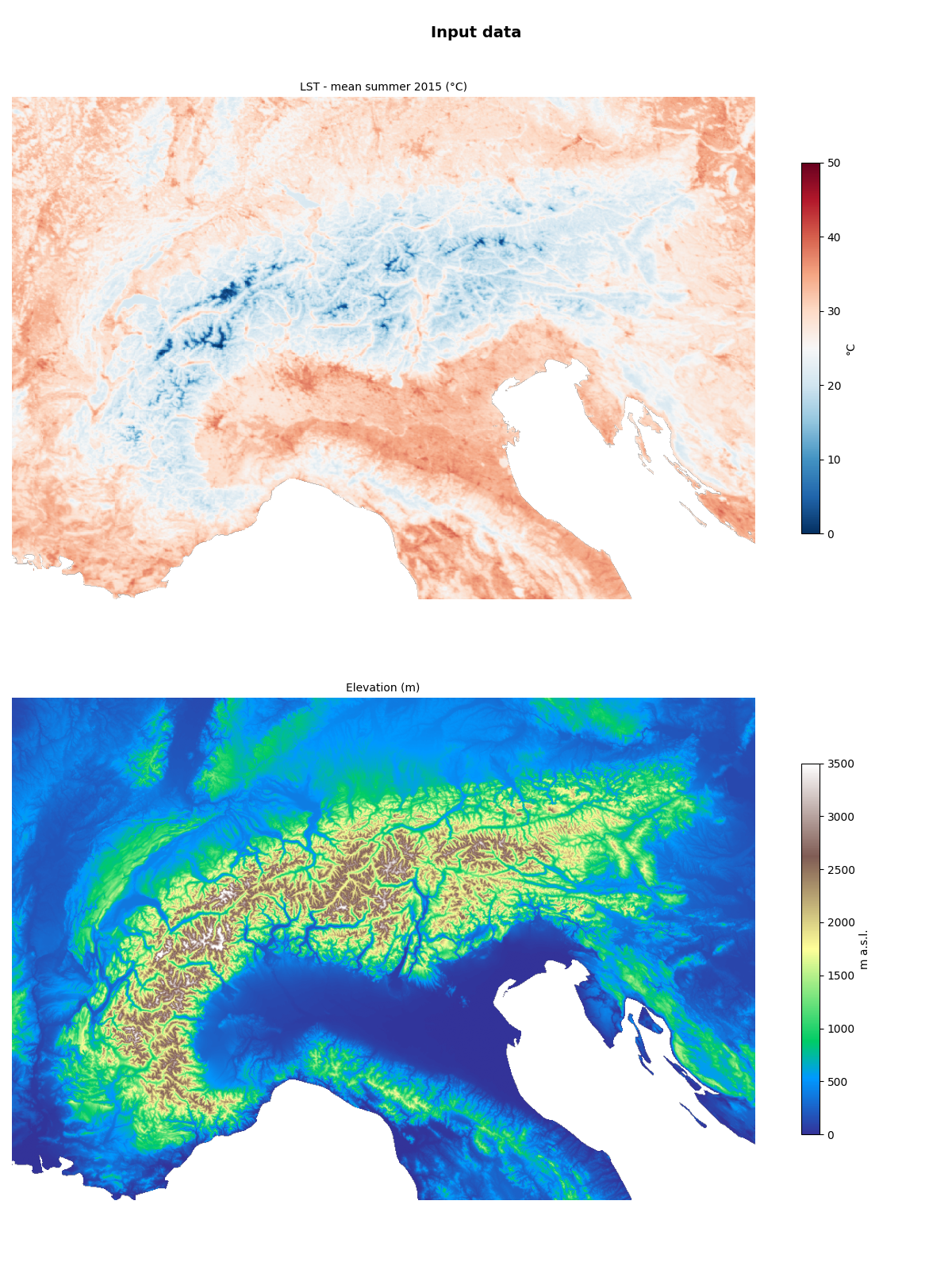
We load two raster datasets covering the European Alps at ~1 km resolution:

• LST - MODIS mean summer land surface temperature (°C)

• Elevation - Copernicus DEM 90 m (aggregated to 1 km)

base_dir =  os.getcwd()

lst_file_org  = os.path.join(base_dir, "../data/example/lst_day_mean_summer_2015_MODISLST8D_alps.tif")
topo_file_org = os.path.join(base_dir, "../data/example/elevation_mean_COP90_alps.tif")

# Work on copies so the originals are never altered
lst_file  = os.path.join(base_dir, "../data/example/_tmp_lst_diff_alps.tif")
topo_file = os.path.join(base_dir, "../data/example/_tmp_elevation_diff_alps.tif")
shutil.copy(src=lst_file_org,  dst=lst_file)
shutil.copy(src=topo_file_org, dst=topo_file)

'/home/docs/checkouts/readthedocs.org/user_builds/georacoon/checkouts/stable/examples/../data/example/_tmp_elevation_diff_alps.tif'

Get working with the Source and Band objects from riogrande, and set a tag for the elevation band we want to use

# Land Surface Temperature
lst_source  = Source(path=lst_file)
lst_profile = lst_source.import_profile()
lst_band    = Band(source=lst_source, bidx=1)

# Elevation
topo_source  = Source(path=topo_file)
topo_profile = topo_source.import_profile()

elev_cat = "elevation_mean"
topo_source.set_tags(bidx=1, tags=dict(category=elev_cat))      # set a tag
elev_band = topo_source.get_band(category=elev_cat)

Set some general paremeters (for parallelization etc. for later use)

params     = dict(nbrcpu=6)
block_size = (200, 200)
data_type  = np.float32

A shared helper for all maps in this example, using Source and Band with get_data() to read the pixel array

def show_map(ax, file, title, limits, cmap="RdBu_r", label="°C", bidx=1,
             add_colorbar=True):
    src = Source(path=file)
    band = Band(source=src, bidx=bidx)
    data = band.get_data()
    ax.set_axis_off()
    img = ax.imshow(data, cmap=cmap, vmin=limits[0], vmax=limits[1])
    ax.set_title(title, fontsize=10)
    if add_colorbar:
        plt.colorbar(img, ax=ax, label=label, shrink=0.6)
    return img

The raw inputs look like this:

fig, axes = plt.subplots(2, 1, figsize=(12, 16))
show_map(axes[0], lst_file_org,  "LST - mean summer 2015 (°C)", limits=(0, 50))
show_map(axes[1], topo_file_org, "Elevation (m)", limits=(0, 3500),
         cmap="terrain", label="m a.s.l.")
fig.suptitle("Input data", fontweight="bold", fontsize=14)
fig.tight_layout()
plt.show()

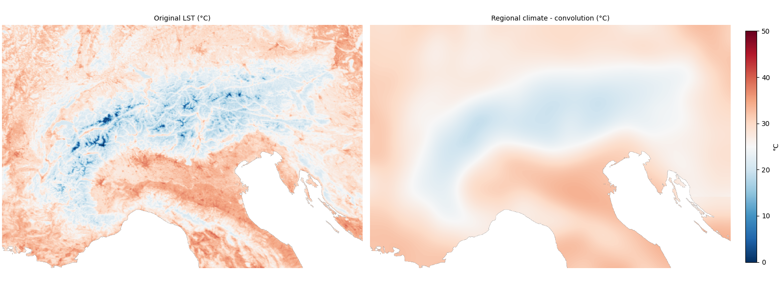
Step 1 - Remove the Regional Climate Signal from LST

A large-kernel Gaussian filter (σ = 30 km) smooths the LST image to capture regional climate variation. Subtracting this smooth surface from the original leaves only the local deviation, which is what we eventually want to model.

The choice of σ reflects the spatial scale at which we consider climate to be “regional”. A larger σ preserves more large-scale structure in the residual; a smaller σ removes less.

# We are setting the sigma in the CRS units (meters)

kernel_m_sigma     = 30_000   # sigma in meters
resolution         = 1_000    # pixel size in meters
kernel_pixel_sigma = kernel_m_sigma / resolution

params_filter = dict(
    sigma=kernel_pixel_sigma,
    truncate=3,               # cut kernel at 3 σ
    preserve_range=True,
)

Prepare the dataset objects for the filter …

lst_conv_file   = os.path.join(base_dir,
                               f"../data/example/_tmp_lst_conv_{kernel_m_sigma}m_alps.tif")
lst_conv_source = Source(path=lst_conv_file, profile=lst_profile)
lst_conv_source.init_source(overwrite=True)
lst_conv_band   = Band(lst_conv_source, bidx=1)

Initiating empty file
        "/home/docs/checkouts/readthedocs.org/user_builds/georacoon/checkouts/stable/examples/../data/example/_tmp_lst_conv_30000m_alps.tif"

… and perform the filter operation with apply_filter(), using bpgaussian() as the filter kernel.

cvpara.apply_filter(
    source=lst_source,
    output_file=lst_conv_file,
    block_size=block_size,
    data_in_range=None,
    data_as_dtype=data_type,
    data_output_range=None,
    img_filter=bpgaussian,
    filter_params=params_filter,
    filter_output_range=None,
    output_dtype=data_type,
    output_range=None,
    selector_band=None,
    **params,
)

total_duration=0.8672178540000459

'/home/docs/checkouts/readthedocs.org/user_builds/georacoon/checkouts/stable/examples/../data/example/_tmp_lst_conv_30000m_alps.tif'

Subtract the filtered band from the LST band using subtract() (inplace). The LST band now holds the local anomaly.

lst_band.subtract(band=lst_conv_band)

The thw panels below show original LST and the regional signal captured by the convolution

# Figure 1: Original LST and Regional climate convolution
fig1, axes1 = plt.subplots(1, 2, figsize=(16, 6), constrained_layout=True)
img1 = show_map(axes1[0], lst_file_org, "Original LST (°C)", limits=(0, 50),
                add_colorbar=False)
img2 = show_map(axes1[1], lst_conv_file, "Regional climate - convolution (°C)",
                limits=(0, 50), add_colorbar=False)
cbar1 = fig1.colorbar(img1, ax=axes1.ravel().tolist(), label="°C", shrink=0.8,
                      pad=0.02)
plt.show()

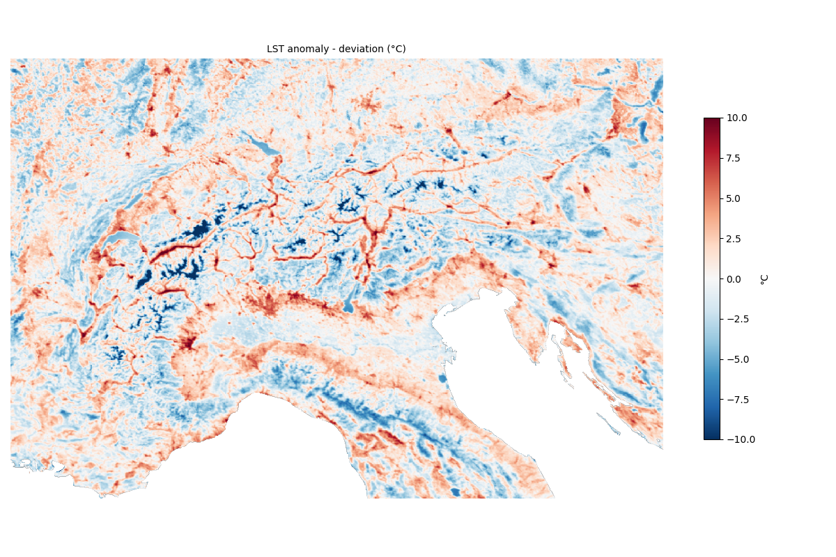
What we will actually model is the anomaly, i.e. the difference between those two:

# Figure 2: LST anomaly
fig2, ax2 = plt.subplots(figsize=(12, 8))
show_map(ax2, lst_file, "LST anomaly - deviation (°C)", limits=(-10, 10))
fig2.tight_layout()
plt.show()

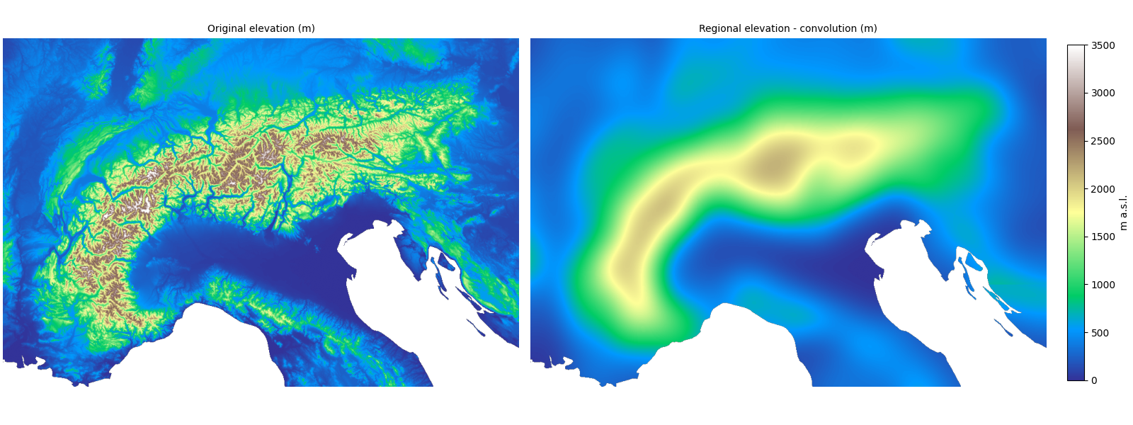
Step 2 - Remove the Regional Elevation Signal

For the same reason, elevation must also be expressed as a local deviation from the regional mean. Without this, a high plateau would have high absolute elevation but zero local anomaly, masking the signal we care about.

# Again we prepare the data ...

elev_conv_file   = os.path.join(base_dir,
                                f"../data/example/_tmp_elev_conv_{kernel_m_sigma}m_alps.tif")
elev_conv_source = Source(path=elev_conv_file, profile=topo_profile)
elev_conv_source.init_source(overwrite=True)
elev_conv_band   = Band(elev_conv_source, bidx=1)

Initiating empty file
        "/home/docs/checkouts/readthedocs.org/user_builds/georacoon/checkouts/stable/examples/../data/example/_tmp_elev_conv_30000m_alps.tif"

… and run the filter using the same parameter as above.

cvpara.apply_filter(
    source=topo_source,
    output_file=elev_conv_file,
    bands=[elev_band],
    block_size=block_size,
    data_in_range=None,
    data_as_dtype=data_type,
    data_output_range=None,
    img_filter=bpgaussian,
    filter_params=params_filter,
    filter_output_range=None,
    output_dtype=data_type,
    output_range=None,
    selector_band=None,
    **params,
)

total_duration=0.8686541850001959

'/home/docs/checkouts/readthedocs.org/user_builds/georacoon/checkouts/stable/examples/../data/example/_tmp_elev_conv_30000m_alps.tif'

We know have a map that represent the regional mean elevation:

# Figure 1: Original elevation and Regional elevation convolution
fig1, axes1 = plt.subplots(1, 2, figsize=(16, 6), constrained_layout=True)
img1 = show_map(axes1[0], topo_file_org, "Original elevation (m)",
                limits=(0, 3500), cmap="terrain", label="m a.s.l.",
                add_colorbar=False)
img2 = show_map(axes1[1], elev_conv_file, "Regional elevation - convolution (m)",
                limits=(0, 3500), cmap="terrain", label="m a.s.l.",
                add_colorbar=False)
cbar1 = fig1.colorbar(img1, ax=axes1.ravel().tolist(), label="m a.s.l.",
                      shrink=0.8, pad=0.02)
plt.show()

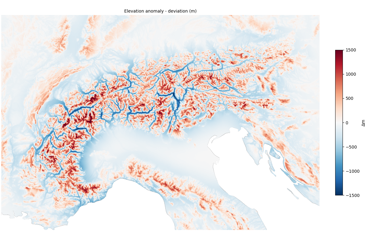
Now we subtract the convolution from the elevation band to obtain the elevation anomaly - local height above (positive) and below (negative) the regional mean surface:

elev_band.subtract(band=elev_conv_band)
# Figure 2: Elevation anomaly
fig2, ax2 = plt.subplots(1, 1, figsize=(12, 8), constrained_layout=True)
show_map(ax2, topo_file, "Elevation anomaly - deviation (m)",
         limits=(-1500, 1500), cmap="RdBu_r", label="Δm")
plt.show()

Step 3 - Fit the Lapse-Rate Model

We now regress the LST anomaly on the elevation anomaly using a pixel-wise ordinary least squares model (no intercept). The fitted coefficient β directly gives the lapse rate in °C m⁻¹.

Let’s create a mask with compute_mask(), so we are only fitting relevant data (not np.nan). We will then tell the Band object to use the mask from the source via set_mask_reader() (not a band specific mask - which is also possible).

rgpara.compute_mask(
    topo_source,
    bands=[elev_band],
    logic="all",
    nodata=np.nan,
    block_size=block_size,
    **params,
)
elev_band.set_mask_reader(use="source")

compute_mask - source=Source(path=/home/docs/checkouts/readthedocs.org/user_builds/georacoon/checkouts/stable/examples/../data/example/_tmp_elevation_diff_alps.tif, exists: True)

Collect the predictors for the model fitting (here only 1), and fit the model with compute_weights() to compute the weights for the predictors.

predictors = [elev_band]

band_weight = lfpara.compute_weights(
    response=lst_band,
    predictors=predictors,
    block_size=block_size,
    include_intercept=False,
    as_dtype=data_type,
    limit_contribution=0.0,
    no_data=np.nan,
    sanitize_predictors=True,
    return_linear_dependent_predictors=True,
    verbose=False,
    **params,
)

Creating selector...
prepare_selector - bands=(Band(tags={}), Band(tags={'category': 'elevation_mean'}))
Check consistency of remaining predictor data...
check_predictor_consistency - predictors=[Band(tags={'category': 'elevation_mean'})]
Calculate X.T @ X...
get_XT_X - response=Band(tags={}), predictors=(Band(tags={'category': 'elevation_mean'}),)
Check linear dependency...
Inverting X.T @ X...
Calculate Y @ X.T @ y (optimal weights)...
get_optimal_betas - response=Band(tags={}), predictors=(Band(tags={'category': 'elevation_mean'}),)

Get the specific results from the returned β values. (Remember no intercept was fitted, which would be in position 0 here the list)

beta_elev  = band_weight[elev_band]
lapse_rate = beta_elev * 1000   # °C m⁻¹ → °C km⁻¹

Lapse Rate Result

The fitted coefficient gives us our lapse rate estimate. Literature reports the annual mean lapse rate in the European Alps at −5.4 to −5.8 °C km⁻¹ (Rolland 2003). Our summer-only estimate is expected to sit at the warmer end of that range or slightly above, as dry-adiabatic conditions dominate in summer.

lit_low, lit_high = -5.8, -5.4   # °C km⁻¹, literature range

print(f"Estimated lapse rate:    {lapse_rate:.2f} °C km⁻¹")
print(f"Literature range (Alps): {lit_low} to {lit_high} °C km⁻¹")

fig, ax = plt.subplots(figsize=(4, 2.5))
ax.plot([-5, -6], [0, 0], color="lightgray", linestyle="dotted", linewidth=1.5,
        zorder=1)
ax.plot([lit_low, lit_high],  [0, 0],         color="black", linewidth=2,
        zorder=2)
ax.plot([lit_low, lit_low],   [-0.05, 0.05],  color="black", linewidth=2,
        zorder=2)
ax.plot([lit_high, lit_high], [-0.05, 0.05],  color="black", linewidth=2,
        zorder=2, label=f"Literature range ({lit_low} to {lit_high} °C km⁻¹)")
ax.plot(lapse_rate, 0, "x", color="darkred", markersize=10, markeredgewidth=2.5,
        zorder=3, label=f"This study: {lapse_rate:.2f} °C km⁻¹")
ax.set_xlabel("Lapse rate (°C km⁻¹)")
ax.set_xlim(-6, -5)
ax.set_yticks([])
ax.set_ylim(-0.3, 0.3)
ax.legend(fontsize=8, loc="upper left")
ax.set_title("Estimated vs. literature lapse rate")
fig.tight_layout()
plt.show()

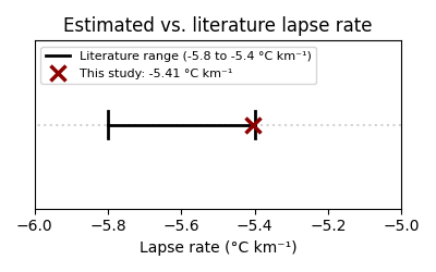
Estimated lapse rate:    -5.41 °C km⁻¹
Literature range (Alps): -5.8 to -5.4 °C km⁻¹

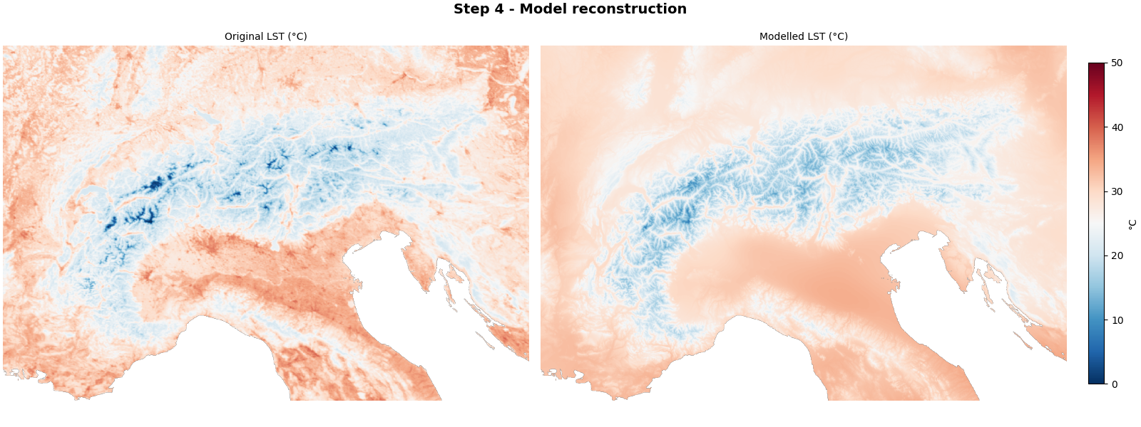
Step 4 - Reconstruct the Full Model

compute_model() reconstructs the full spatial prediction from the fitted weights. We then add the regional climate signal back via add(). The result should approximate the original LST.

model_file     = os.path.join(base_dir,
                              f"../data/example/_tmp_model_conv_{kernel_m_sigma}_m.tif")
model_data_tif = lfpara.compute_model(
    predictors=predictors,
    optimal_weights=band_weight,
    output_file=model_file,
    block_size=block_size,
    profile=lst_profile,
    verbose=False,
    **params,
)

# Add regional climate back → full modelled LST
model_source = Source(path=model_data_tif)
model_band   = model_source.get_band(bidx=1)
model_band.add(band=lst_conv_band)

total_duration=0.22927027200057637
maximal duration of single job: max(job_timers)=0.08886437799810665

Comparing the original and modelled LST:

fig, axes = plt.subplots(1, 2, figsize=(16, 6), constrained_layout=True)
img1 = show_map(axes[0], lst_file_org, "Original LST (°C)", limits=(0, 50),
                add_colorbar=False)
img2 = show_map(axes[1], model_file, "Modelled LST (°C)", limits=(0, 50),
                add_colorbar=False)
cbar = fig.colorbar(img1, ax=axes.ravel().tolist(), label="°C", shrink=0.8,
                    pad=0.02)
fig.suptitle("Step 4 - Model reconstruction", fontweight="bold", fontsize=14)
plt.show()

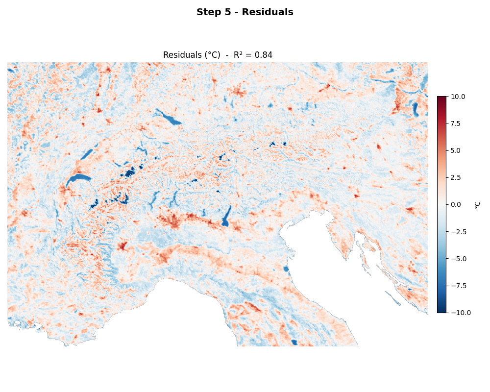
Step 5 - Accuracy Assessment & Residuals

We quantify model performance with RMSE and R² using calculate_rmse() and calculate_r2(). prepare_selector() builds a shared valid-pixel mask across response and predictors. Two variants are reported:

• Residual - how well the lapse-rate component alone explains the LST anomaly (what was directly fit).

• Overall - how well the complete model (convolution + lapse rate) explains the original LST.

lst_org_source = Source(path=lst_file_org)
lst_org_band   = Band(lst_org_source, bidx=1)
rgpara.compute_mask(
    lst_org_source,
    bands=[lst_org_band],
    logic="all",
    nodata=np.nan,
    block_size=block_size,
    **params,
)
lst_org_band.set_mask_reader(use="source")
_selector_all = rgpara.prepare_selector(lst_org_band, *predictors,
                                        block_size=block_size)

rmse = lfpara.calculate_rmse(response=lst_band, model=model_data_tif,
                             selector=_selector_all, block_size=block_size,
                             **params)
r2_resid = lfpara.calculate_r2(response=lst_band, model=model_data_tif,
                               selector=_selector_all, block_size=block_size,
                               **params)
r2_full = lfpara.calculate_r2(response=lst_org_band, model=model_data_tif,
                               selector=_selector_all, block_size=block_size,
                               **params)

print(f"Residual model - RMSE: {rmse:.2f} °C  |  R²: {r2_resid:.2f}")
print(f"Full model     - RMSE: {rmse:.2f} °C  |  R²: {r2_full:.2f}")

# Residual map
resid_file   = os.path.join(base_dir,
                            f"../data/example/_tmp_resid_model_conv_{kernel_m_sigma}_m.tif")
resid_source = Source(path=resid_file, profile=lst_profile)
resid_source.init_source(overwrite=True)
resid_band   = Band(source=resid_source, bidx=1)
lst_org_band.subtract(band=model_band, out_band=resid_band)

compute_mask - source=Source(path=/home/docs/checkouts/readthedocs.org/user_builds/georacoon/checkouts/stable/examples/../data/example/lst_day_mean_summer_2015_MODISLST8D_alps.tif, exists: True)
prepare_selector - bands=(Band(tags={}), Band(tags={'category': 'elevation_mean'}))
Residual model - RMSE: 27.52 °C  |  R²: -117.94
Full model     - RMSE: 27.52 °C  |  R²: 0.84
Initiating empty file
        "/home/docs/checkouts/readthedocs.org/user_builds/georacoon/checkouts/stable/examples/../data/example/_tmp_resid_model_conv_30000_m.tif"

Residuals reveal where the model over- or under-predicts - for example, urban heat islands or cold air pooling around water bodies:

fig, ax = plt.subplots(1, 1, figsize=(10, 8))
src = Source(path=resid_file)
band = Band(source=src, bidx=1)
data = band.get_data()
ax.set_axis_off()
img = ax.imshow(data, cmap="RdBu_r", vmin=-10, vmax=10)
ax.set_title(f"Residuals (°C)  -  R² = {r2_full:.2f}", fontsize=12)

# Compact colorbar (narrower width to give more space to plot)
cbar = plt.colorbar(img, ax=ax, label="°C", shrink=0.6, aspect=25, pad=0.02,
                    fraction=0.046)
fig.suptitle("Step 5 - Residuals", fontweight="bold", fontsize=14)
fig.tight_layout()
plt.show()